As a data scientist, my job revolves around three simple themes: generating data, understanding data, and communicating my understanding of the data to others. Within these themes, the act of visualising data is an essential element in successfully understanding and communicating data - pictures speak a thousand words after all. However, as a scientist, I am not just communicating data to other scientists in my field, but also to scientists in other fields, or perhaps to an audience with no specialist scientific background, which poses a challenge: how can I build visualisations that can easily be tuned to different audiences?
Over the course of two blog posts, I will demonstrate a software tool, the ggplot2 package in R, that has become an indispensable part of every data visualisation I generate, and how its flexibility allows us to tailor our visualisations to specific audiences. This blog post will not be a tutorial for new users as there are plenty of those already (for example, see here), but through five key concepts will demonstrate how flexible ggplot2 can be.
Why visualise data in R and what is the ggplot2 package?
In short, because you're probably already using R, and if not, maybe you should be! The R programming language was originally conceived as a language 'developed by statisticians, for statisticians'. Its open-source and community-orientated developer base has meant that R has become a hugely versatile and powerful language for all sorts of analytical tasks. The chances are, no matter what sort of analyses you wish to conduct or which sort of data you work with, R can probably do it - and if not, you can write your own code to fix these shortcomings!
R already has many functions and capabilities to visualise your data. If you've ever accessed any sort of beginner tutorials or course materials, then you've probably used functions like plot(), boxplot(), or hist() to generate basic data visualisations. The ggplot2 package takes data visualisation in R to another level. Not only does it automatically take care of some of the mundane aspects of building plots that R's base graphics don't (having to manually build figure legends and setting margin sizes are two that I find particularly irksome!), but ggplot2 allows for a high-degree of customisation, making it a very versatile and flexible tool for data visualisation. I shan't go too far into the history and development of the ggplot2 package (if you want to, you can read about it here), suffice to say that it has become one of the most popular R packages, having been downloaded > 3.2 million times in the previous month alone!
Concept 1 - Plots are built in layers
As with any R package, we first need to download it, install it, and load it from our library. For this demo, we will also use the penguins dataset which is available in the palmerpenguins package.
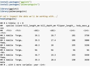
The key thing to be aware of when building plots using ggplot2 is that they are built in layers. The underlying data is always the first layer, and we build up from there. We define which columns or variables from our data we wish to show in our plot inside the aesthetics (aes() function).

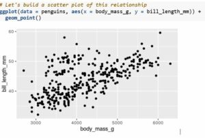
Next, we must add some 'geometric objects' or 'geoms' for short. These determine what is actually plotted, and we can combine multiple geoms by layering them atop each other. Order is important when we combine multiple geoms - geoms that appear first in our code will be plotted first, with subsequent geoms layered on top. Let's have a look at an example...
Now let's build the same plot, but with a fitted statistical relationship over the top, by adding another geom.
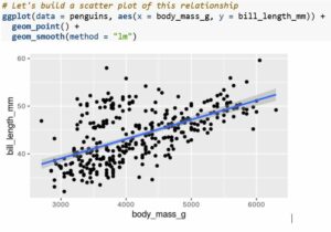
See how the fitted line has been plotted over the top of the scatter points? If we reversed the order of those two geoms, the points would be plotted over the top of the fitted line.
Concept 2 - Colours and point shapes and linetypes, oh my!
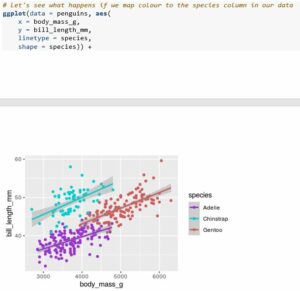
Whilst creating simple plots like the one above is often useful, there are often cases where our data are more complex and may have one or more grouping variables present that we wish to show. ggplot2 makes it very easy to map these additional factors to various aesthetic attributes of our plot. Let's consider the previous plot we made - whilst the relationship between body mass and bill length seems simple enough, we also have additional information on the species of penguin measured that we might wish to show, so we can look at some ways we might show this extra information.
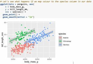
Note that both the colour of the scatter points and the fitted lines changed, and that a legend automatically appears to the right of our plot. We can also try mapping point shapes and/or linetypes to categorical factors in our data.
By providing a vector of colour names to the values argument, we can easily override the default colours. If you want to see some of the possible colours you can use in R, check out this document. Similarly, we could override the point shapes using the scale_shape_manual() function, like so:
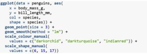
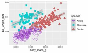
Here, I changed the point shapes by specifying which of these shapes I wanted. Note also that I made the points bigger to highlight the differences by adjusting the size argument inside the geom_point() function.
Summary
So that wraps up part one of this two-part post on visualising data in R. Within this post, we've seen how to build a plot using the ggplot2 package by building up the layers of the plot, and how we have almost total control over how these layers appear through functions to customise the aesthetics of our plot. In the next post, we'll see how we can fine-tune the appearance of our plot and how extension packages can be used to elevate our plots to another level.